Nobile Engineering blog

You have set up a video processing pipeline or simply have a camera attached to a Raspberry Pi and want to be able to watch the video from a browser?

Streaming live video can be done using several protocols,  among the most popular we have HTTP, RTMP and RTSP.

HTTP is the most widely used protocol to serve static video but can also be used for live content.

RTMP was initially developed by Macromedia (Adobe) to enable streaming of audio and video between a server and a Flash player and is a TCP-based protocol.

RTSP (Real Time Streaming Protocol) was developed by  RealNetworks, Netscape, and Columbia University and is not supported natively by most browsers.

Ideally the solution would enable anyone with a working browser, including smartphones and tablets,  to be able to consume the video. A good option is to use  HTTP Live Streaming (HLS). HLS was developed by Apple Inc. and according to Wikipedia:

“works by breaking the overall stream into a sequence of small HTTP-based file downloads, each download loading one short chunk of an overall potentially unbounded transport stream. A list of available streams, encoded at different bit rates, is sent to the client using an extended M3U playlist.”

By being based on standard HTTP, it is not being blocked by firewalls or proxys that let standard HTTP traffic go through. The drawback is the relatively high latency compared to other protocols.

The solution proposed here is to use the RTMP protocol to send the stream form the camera to the cloud and  then convert it to HLS using NGINX. If you want to use Apache or another web server to serve the stream this can be done easily.

NGINX has a very nice rtmp module that is perfectly suited for the task.  In order to use it we are going to build NGINX with support for it.

$ sudo apt-get install build-essential libpcre3 libpcre3-dev libssl-dev
$ git clone git://github.com/arut/nginx-rtmp-module.git
$ wget http://nginx.org/download/nginx-1.12.0.tar.gz
$ tar xzf nginx-1.12.0.tar.gz
$ cd nginx-1.12.0
$ ./configure --with-http_ssl_module --add-module=../nginx-rtmp-module
$ make
$ sudo make install

This will install NGINX in /usr/local.
To start the service

$ sudo /usr/local/nginx/sbin/nginx

while to stop it:

$ sudo /usr/local/nginx/sbin/nginx -s stop

If you are using already a web server, it’s better to modify the nginx configuration file before starting it.
Open the file “/usr/local/nginx/conf/nginx.conf” with an editor and enable RTMP and HLS following the example below (note that i used the user www-data since I have apache installed that uses www-data as user):

user  www-data;
worker_processes  1;

error_log  logs/error.log debug;

events {
    worker_connections  1024;
}

http {
     sendfile off;
     tcp_nopush on;
     directio 512;
     default_type  application/octet-stream;
     server {
        listen       localhost:2222;
        server_name  $hostname;

        location / {
                root /var/nginx_www;
                index index.html;
        }
        location /hls {
        # Disable cache
        add_header Cache-Control no-cache;

        # CORS setup
        add_header 'Access-Control-Allow-Origin' '*' always;
        add_header 'Access-Control-Expose-Headers' 'Content-Length';

        # allow CORS preflight requests
        if ($request_method = 'OPTIONS') {
            add_header 'Access-Control-Allow-Origin' '*';
            add_header 'Access-Control-Max-Age' 1728000;
            add_header 'Content-Type' 'text/plain charset=UTF-8';
            add_header 'Content-Length' 0;
            return 204;
        }

        types {
            application/vnd.apple.mpegurl m3u8;
            video/mp2t ts;
        }

        root /tmp/hls;
        }

        # rtmp stat
        location /stat {
            rtmp_stat all;
            rtmp_stat_stylesheet stat.xsl;
        }
        location /stat.xsl {
            # you can move stat.xsl to a different location
            root /usr/build/nginx-rtmp-module;
        }

        # rtmp control
        location /control {
            rtmp_control all;
        }

        error_page   500 502 503 504  /50x.html;
        location = /50x.html {
            root   html;
        }
    }
}

rtmp {
    server {
        listen localhost:1935;
        ping 30s;
        notify_method get;

        application live {
            live on;

            # sample HLS
            hls on;
            hls_path /tmp/hls;
            hls_sync 100ms;
            hls_fragment 3;
            hls_playlist_length 60;
            allow play all;
        }
    }
}

With this configuration both the http server and the rtmp servers will listen on localhost with the http on port 2222 and rtmp on the standard 1935.
The HLS files and playlist will be generated and put in “/tmp/hls” (specified by hls_path /tmp/hls;)
To push the stream to the server from a device we can use an ssh tunnel on the port 1935 and map the device-local port 1935 to the remote server port 1935

$ ssh -L1935:remoteserver:1935

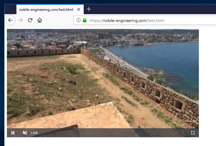
To make the stream accessible by a browser there is a javascript video player video.js that can be embedded in a normal html page.

<!DOCTYPE html>
<html lang="en">
  <head>
    <link href="https://vjs.zencdn.net/7.1/video-js.min.css" rel="stylesheet">
    <script src="https://vjs.zencdn.net/7.1/video.min.js"></script>

  </head>
  <body>
      <video id="player" class="video-js vjs-default-skin"  controls >
        <source src="http://remoteserver.com/hls/mystream.m3u8" type="application/x-mpegURL" />
      </video>
  
  <script>
    var options, video;

    options = {
      autoplay: true,
      muted: true
    };

    video = videojs('player', options);

  </script>

  </body>
</html>

the line with

<source src="http://remoteserver.com/hls/mystream.m3u8" type="application/x-mpegURL" /> 

tells the player where the stream source is located.
In NGINX the rtmp application is called live and the name of the .m3u8 file is mystream.m3u8.
This must match the published rtmp stream url

 rtmp://localhost/live/mystream 

Since the stream is composed by regular files that are video fragments, it’s sufficient to expose the directory that contains them to the outside world. For example by creating an alias with apache2, inside the virtualhost conf put

Alias /hls "/tmp/hls"    
<Directory "/tmp/hls">
Options FollowSymLinks
AllowOverride All
Order allow,deny
Allow from all
Require all granted
</Directory>

and ensure that the directory /tmp/hls is accessible by the user with which apache executes.

The example working with apache and the opencv + ffmpeg + rtmp streaming example program to generate the stream

Happy streaming!!!

Do you have a project using OpenCV to process video?
At some point, after your proof-of-concept works,  you want to send the result of the processing in real time to some other device. For example to a VM in the cloud with a web server that can push the stream to a browser. You need to use streaming!

When googling for examples of streaming, the option of using ffmpeg libraries becomes appealing but…

FFmpeg examples are mostly about using the FFmpeg command line tool to produce a stream from a video file, while you want to stream on the fly the cv::Mat frames produced by your code.

Using libavcodec libavformat libavutil libswscale libavfilter and libavdevice is not straightforward. It is fairly easy to have crashes and memory leaks that are extremely time consuming to discover and fix.

After spending some time walking through the FFmpeg code, docs and examples, I decided to implement a little example with basic rtmp streaming functionality and share it in the hope it can save some pain to people wanting to implement streaming from OpenCV based applications.

Here is the github repo with the example.

Feel free to contact me for questions, help or suggestions on how to improve it!

Batch normalization is an important component of Convolutional Neural Networks (CNN). The various improvements it brings, in particular speed and easiness of training, have made the technique widespread. In contrast with convolution operations, that have a high arithmetic intensity (ratio between number of arithmetic operations and data required), batch normalization has a pretty low arithmetic intensity.
This makes batch normalization appear as a non-negligible fraction of the time spent in CNN inference despite the relatively low arithmetic operation count.
It is well known to people concerned with performance in particular in the computer hardware and high performance computing (HPC) communities that memory bandwidth and latency are an important bottleneck in existing computing system (the memory wall). The 3 or 4 level cache hierarchy and associated hardware complexity and power requirements in current processors would have no reason to exist if the main  memory could achieve the same level of performance of the caches. It’s interesting to look at the typical latency of operations that are thought to be expensive and compare those with memory accesses that miss the cache.

In the subconscious mind of many programmers floating point operations have high cost while memory operations are virtually free. Nothing is more far from reality. As an example we can look at the latency in clock cycles needed to compute a square root, an operation for which very clever and famous approximate implementations have been produced for game engines. Let’s look at this amazing  document : For example SQRTSS on an AMD Bulldozer takes 14-15 clock cycles, while latency to access memory is of the order of ~100 ns or more which at 3GHz translates to ~300 cycles. This is a whopping 20 times the cost of a costly square root.

This observation should immediately make us think about how our program moves and uses data. Writing fast code is primarily about maximizing the amount of useful work done with the data we have loaded into the caches.

In order to manipulate arrays it is common practice to use high level functions that execute very simple operations like element-wise sum, multiply or multiply an array by a scalar, instead of using loops. While this is a good approach in interpreted languages like python (in which a loop can be expensive and it’s preferred to call a function implemented in native code) it might not be always the best option at the C/C++ level.

As an example let’s take a simple sequence of operations we want to do on a few arrays. I will assume the vectors are big and do not fit into the small cache available.

\(A \leftarrow A+B\times d + C\times e \)
where \(A, B \) and \(C\) are arrays and \(d, e\) are scalars.

in pseudo-code a typical implementation might look like:

tmp1 = array_scale(B, d)
tmp2 = array_scale(C, e)
tmp3 = array_sum(tmp1, tmp2)
A = array_sum(A, tmp3)

“Not too bad!” you would think,  since array_scale and array_sum are highly optimized functions written by experts. While it is certainly true that array_sum and array_scale are well optimized, and very likely reach the maximum performance obtainable on the system, this alone does not guarantee that the implementation above cannot be improved. Actually it can be greatly improved.
At line 1 we read 1 array and we write out 1 array, for a total of 2 arrays moved. At line 2 the same happens while at line 3 we have 2 array reads and 1 array write, at line 4 we have 2 array reads and 1 array write. If we sum all the movements we get a grand total of 10 array moves between main memory and the execution units. We have also 3 temporary arrays. This is a bit strange isn’t it? In our expression we only have 3 arrays on the right and 1 on the left, which gives 4. How can we get a more efficient implementation? The answer is simple! Let’s use a good old-fashioned loop!

for(i=0;i<n;i++) {
  A[i] = A[i] + B[i]*d + C[i]*e; 
}

What have we gained? Now the computation is on 1 line, it’s clear to read, no temporary arrays are needed and we have moved 4 arrays, as necessary for our expression, not more.
It’s extremely likely that this implementation is faster than the previous one even if we have not used carefully tuned functions. This is because our computation is memory-bandwidth bound on all modern architectures. The simple loop implementation above is likely to reach the maximum bandwidth available to a core on an typical out-of-order processor with a good hardware prefetcher. The compiler is also likely to optimize well the loop if we are careful enough to make clear that the arrays A, B and C are disjoint. The same maximum bandwidth will be reached by the highly optimized functions called in the first implementation but in that case we have moved 10 arrays! So the speedup \( s \) of the “loop” implementation compared to the “function call” is approximately:

\(
s \approx \frac{10}{4} = 2.5 .
\)Let’s have a look at batch normalization now! From the original paper, we look at the expression defining batch norm:

\( \hat{x}_i = \frac{x_i – \mu_B}{\sqrt{\sigma^2_B + \epsilon}} \)
where \( \mu_B \) is the mean and \( \sigma^2_B \) is the variance of the inputs.
They also add a scale and shift operation:

\(
y_i = \gamma \cdot \hat{x}_i + \beta
\)
The authors, to shine more light on the math, clearly express in the paper that:

Since the means and variances are fixed during inference,
the normalization is simply a linear transform applied to
each activation. It may further be composed with the scaling
by γ and shift by β, to yield a single linear transform

Let’s now “compress” the entire batch norm to a very simple linear transform as claimed and derive the parameters:

\(
y_i = \gamma \cdot \frac{x_i – \mu_B}{\sqrt{\sigma^2_B + \epsilon}} + \beta
\)
Since \( \gamma \), \( \mu_B \), \( \sigma^2_B \), and \( \epsilon \) are constants known ahead of running inference, we can simplify the expression and get:

\(
y_i = \eta x_i + \omega
\)
With \( \eta = \frac{\gamma}{\sqrt{\sigma^2_B + \epsilon}} \) and \( \omega = –
\frac{\gamma\mu_B}{\sqrt{\sigma^2_B + \epsilon}} + \beta \).

How do we implement batch normalization for inference then?
A loop can do the job very well. In this case also a BLAS function called AXPY together with a couple of other calls might do the job. Since AXPY will destroy the input data replacing it with the output it is not a perfect fit for our operation. We can quickly code the straightforward loop:

for(i=0;i<n;i++) {
  output[i] = input[i]*eta + omega; 
}

I had a look at the batch norm implementation in a couple of frameworks, Caffe and clDNN from Intel. Caffe does not distinguish well between training and inference time so it does not take real advantage of the situation. While clDNN does a great job, it still does calculations and data movements that can be avoided at inference time.
\( \eta \) and \( \omega \) can be computed at model loading ahead of time so the only calculation that needs to be done at every inference is the simple loop above.

In my simple inference engine the batch norm implementation (Caffe-compatible) is merged with ReLU activation to further reduce memory traffic. The unoptimized, but already well performing kernel looks like:

static inline void bn_arrays(float * __restrict__ data_in, float * __restrict__ data_out, size_t n, float nrm, float mn_nrm, bool relu)
{
    if(relu) {
        for(size_t k=0;k<n;k++) {
            data_out[k] = max(data_in[k]*nrm - mn_nrm, 0.0f);
        }
    } else {
        for(size_t k=0;k<n;k++) {
            data_out[k] = data_in[k]*nrm - mn_nrm;
        }
    }
}

We see that in order to reduce memory traffic, we have to give up some code modularity and group operations while looping on data. We might not find in a library the function that does exactly what we need such that we can avoid having a naked loop in our code. Even if we could find it, if the performance is an important factor, the right approach is to measure the performance of different approaches and choose the best one. The way to come up with efficient code is to think in terms of data movement and remember that there is a memory bottleneck.
Code generality and aiming at code reuse are very good principles, but when performance is an important requirement it is not always obvious how to satisfy these often incompatible constraints.
My preference goes to performance, in this case the function is very simple, the logic is straightforward, and I find it more clear than the function-call based implementations.